Modeling & LLMs
A trace-based DSL plus a deterministic compiler beats direct BPMN-XML generation on diagram validity
Master's thesis (TFM) — summary for dissemination
Project Abstract
This is the engineering and evaluation backbone of a Master's thesis (TFM) on generating valid BPMN 2.0 diagrams from natural-language process descriptions with LLMs. Its central thesis: asking a model to emit a small, trace-based textual DSL, which a deterministic compiler then turns into BPMN XML, produces more reliably valid diagrams than asking the same model to emit BPMN XML directly.
The work comprises a DSL compiler, two web apps that use it, a corpus of ~445 tracked model runs, and a reference-free evaluation pipeline that scores both approaches on the same metrics:
- A BPMN engine — DSL → abstract syntax → BPMN model → automatic layout → XML/SVG, plus a validator.
- A research editor — live DSL ↔ canvas, holding the experiment corpus.
- A public landing/demo page — together with the versioned system prompts.
- A Python evaluation pipeline — the ten BPMN metrics M1–M10.
- The written thesis (memoria), the zero-shot harness specification, and the derived-metrics analysis.
1. What BPMN is
BPMN (Business Process Model and Notation) is the OMG standard graphical language for modeling business processes. A BPMN diagram describes how work flows: it is a directed graph of activities (tasks — user, service, manual, business-rule, send/receive, script), events (start, end, intermediate; timer, message, error, signal, escalation, terminate, boundary), gateways that route control flow (exclusive/XOR decisions, parallel/AND splits and joins, event-based gateways), sequence flows wiring those nodes together, pools and swimlanes that say who performs each step, with message flows crossing pool boundaries, data objects / data stores representing the artifacts a process reads and writes.
Crucially, BPMN has two layers. The semantic layer (the process elements above) says what the process is; the diagram-interchange (DI) layer (the diagram, with shapes and waypoints) says where every box and line is drawn. A .bpmn file is XML that must conform to the BPMN 2.0 XSD and, to be openable in tools like bpmn-js, Camunda or Bizagi, must also carry valid DI. This two-layer, schema-constrained nature is exactly what makes direct LLM generation fragile — and is the gap this project targets.
2. Why an intermediate DSL is used
Asking an LLM to write BPMN XML directly is a hard generation target for three compounding reasons:
- It is verbose and redundant. Every node needs a unique ID, every sequence flow must reference valid source/target IDs, and the whole thing must be repeated in the DI layer with coordinates. A single dropped or mismatched ID produces an invalid file.
- Layout is not the model's job, but XML forces it to be. To be importable, the XML needs DI geometry. Models either omit it (file won't open) or hallucinate overlapping coordinates.
- Global structural invariants are easy to violate. Split gateways need matching joins; every node must be reachable; diverging gateways need conditions or a default. These are graph-global properties that token-by-token generation handles poorly.
The project's answer is to reproduce the BPMN Sketch Miner DSL (bpmn-sketch-miner.ai) — a trace-based textual notation — and pair it with our own deterministic compiler. BPMN Sketch Miner is a tool that reconstructs (“mines”) a BPMN model from short textual execution traces; this project re-implements that DSL and its mining behavior as a self-contained engine so it can be driven by an LLM and slotted into a reproducible evaluation pipeline.
Its design philosophy is the meta-rule “think in traces, not in gateways.” Instead of drawing a graph, the author writes execution traces — each end-to-end path through the process as a short paragraph — and lets the miner reconstruct the graph:
- One line, one element; the first word sets the element type (user, service, (timer …), [data], Pool:…).
- Each label appears once in the rendered diagram. Writing the same task name in two traces is how you create a branch or a merge; repeating a name inside one trace is how you create a loop. Gateways are an output of the miner, not an input from the author — XOR splits/joins, loops and event-based gateways are all inferred from the overlap between traces.
- Pools, message flows, boundary events, data objects, parallel branches and reusable fragments round out the surface syntax.
This buys several things that directly attack the failure modes above:
- Validity by construction. Once the DSL parses and passes semantic checks, the compiler emits schema-conformant BPMN with correct IDs and references — the model can no longer produce a malformed-XML file.
- Layout for free. The engine computes orthogonal edge routing, pool/lane placement and DI geometry deterministically, so every output is openable in real BPMN tools.
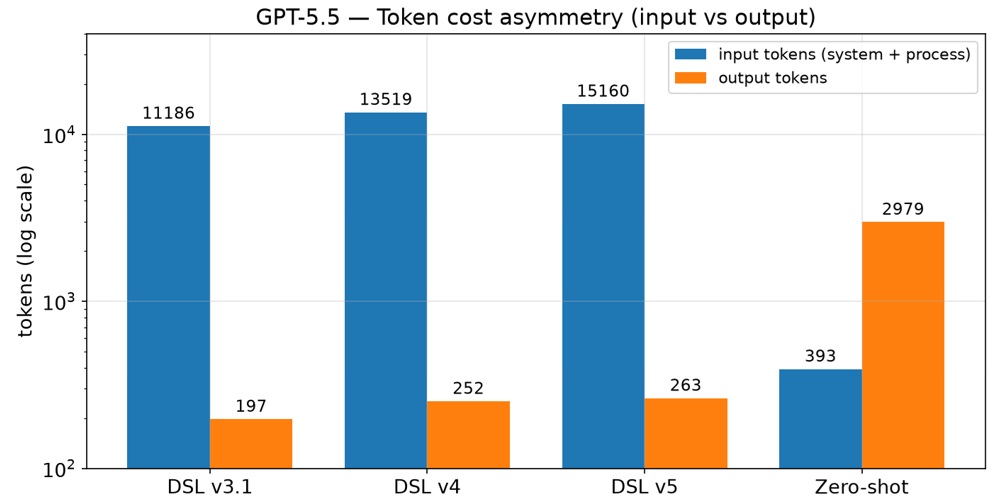
- A much smaller, higher-signal generation target. The model writes ~20 lines of traces instead of hundreds of lines of XML, so its effort goes into getting the process right rather than getting the serialization right.
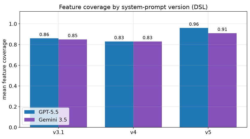
The system prompt is itself a research artifact
It is versioned as a deliberate ablation. The production prompt is v5, and it carries the complete ruleset:
- the structural core — trace-thinking, the seven catalogued anti-patterns, and the anchor-boundary rule that keeps fragment-based compression safe;
- the readability layer (added in v4) — name every decision-gateway question, and name every start and end event so the diagram's trigger and outcomes are explicit at a glance;
- the explicit-pools layer (added in v5) — a named-pools block plus message-flow discipline, which makes the most common multi-pool defect (a control-flow hand-off crossing a pool boundary) a visible, prescriptive warning instead of a silently-wrong diagram.
The structural rules are held byte-stable between versions, so any quality delta is attributable to the single changed layer. v3.1 — the structural-only version — was created for testing purposes, as the ablation baseline against which v4's readability layer and v5's explicit-pools layer are measured. The prompt also documents a three-iteration “Find a Job” failure case and catalogs seven concrete anti-patterns it was hardened against.
3. From pipeline to automatic correction
The end-to-end flow, all sharing a single engine, is:
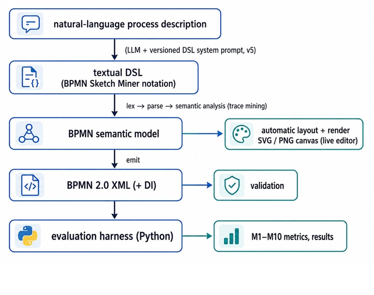
Concretely:
- Authoring / generation. A model is given the DSL system prompt plus a process description (15 synthetic processes spanning easy → medium → hard → stress difficulty). Its output is stored as a tracked experiment with the input, the raw output, and a record of provenance, representation, token estimates and expected features.
- Compile. The miner turns the traces into a BPMN model, serializes it to XML, and adds DI. The editor does this live (DSL on the left, canvas on the right) and headlessly for batch rendering.
- Validate. The validator raises located, prescriptive warnings rather than silently “fixing” illegal structure — illegal edges are kept out of the export so the file stays importable in strict tools.
- Evaluate. The Python pipeline scores every experiment on ten reference-free metrics (no ground-truth diagram needed), through a documented fairness boundary: zero-shot XML is always scored on the raw model output; auto-layout may be applied for visualization only and is never used for scoring. Malformed raw XML gets M1 = 0 and zero scores — it is never repaired before scoring.
- Orchestrate. One command renders missing artifacts and evaluates everything; another drives the DSL-vs-direct-XML comparison. Results are then turned into the research-question figures.
Foundation for automatic error correction
The pipeline is deliberately built so that failures are diagnosable and localized — the precondition for a future closed-loop self-correction stage. Three properties make this tractable:
- The validator produces structured, located diagnostics rather than a binary pass/fail. A warning doesn't just say “invalid” — it names the offending hand-off and prescribes the remedy (“remodel as a message flow”), in the same vocabulary the system prompt uses.
- The failure space is small and catalogued. Because the DSL surface is tiny and the prompt enumerates seven concrete anti-patterns, most failures map onto a known class with a known fix.
- Errors surface at the DSL/compile stage, not buried in thousands of lines of XML. A repair only has to edit ~20 lines of traces.
The natural next step — and the one the architecture is shaped for — is a feedback loop: when the compiler or validator rejects an output or emits warnings, feed those structured diagnostics back to the model (or a rule-based fixer) as a follow-up turn, asking it to repair that specific anti-pattern, and re-compile. Round-tripping a 20-line trace through “compile → read the diagnostic → patch the offending line → recompile” is cheap and convergent, whereas iterating on raw BPMN XML would mean re-emitting the entire serialized graph each round.
4. Evaluation & results
The DSL improves diagram validity
The evaluation is reference-free: ten metrics judge a diagram on its own internal correctness, so no hand-built gold model is required. Scored metrics are normalized to [0, 1]; descriptive ones report raw values without distorting the means.
| Metric | What it measures |
|---|---|
| M1 XML validity | conformance to the BPMN 2.0 XSD |
| M2 structural connectedness | reachability + ID integrity |
| M3 element degree | per-type in/out-degree rules |
| M4 gateway executability | default paths / conditions on diverging gateways |
| M5 label completeness | fraction of elements with a name |
| M8 gateway matching | every split has a type-matched join |
| M6/M7/M9/M10 | size, Cardoso CFC, network complexity (CNC), cyclicity |
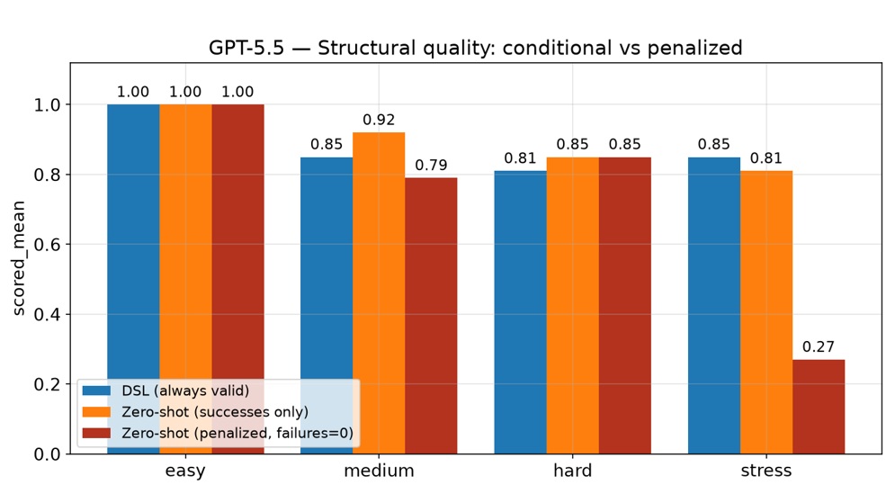
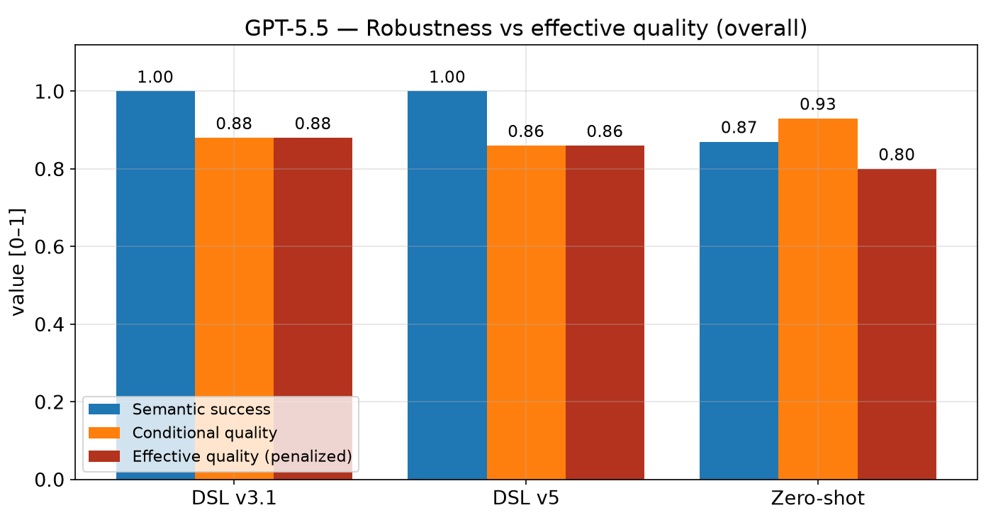
Two aggregates are always read together to avoid survivorship bias: scored_mean (quality over successful runs only) and scored_mean_penalized (failures counted as 0), alongside the semantic_success_rate.
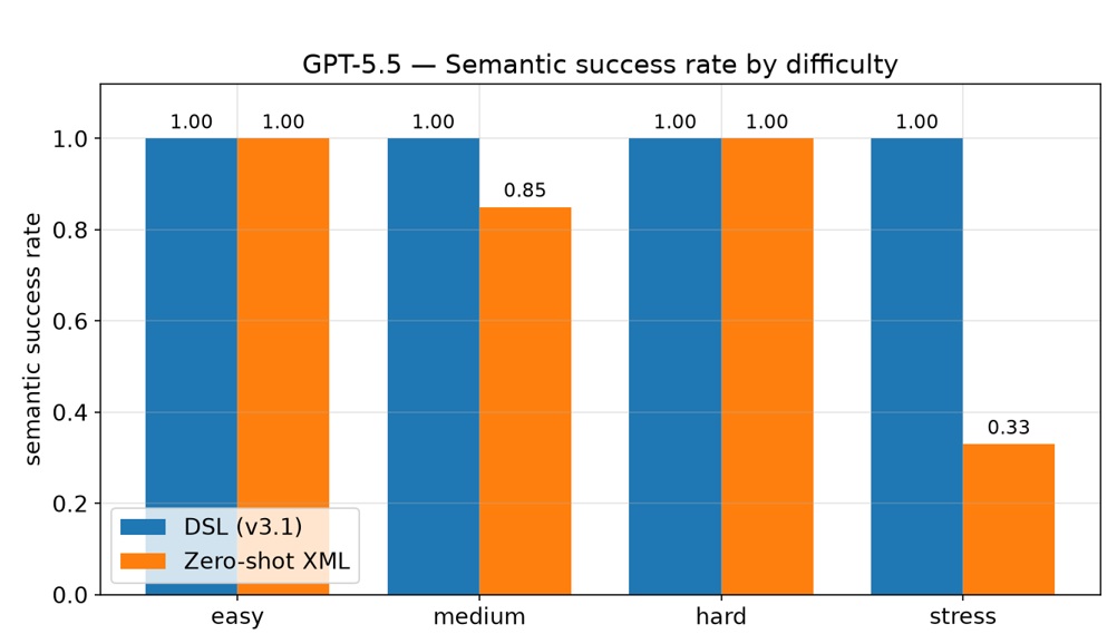
The headline result is about validity
For the DSL path, M1 XML validity is guaranteed conditional on compilation: a DSL that parses always emits schema-valid BPMN with DI. For the direct-XML path it is not — in the tracked corpus, raw zero-shot BPMN-XML was schema-invalid ~13% of the time (validity ≈ 0.87), and on the hardest inputs the direct-XML validity collapses (stress ≈ 0.33). Because every downstream metric is gated on M1, that invalidity propagates: the penalized quality of zero-shot drops well below its conditional quality (≈ 0.91 conditional but ≈ 0.80 penalized overall, and 0.81 → 0.27 on stress cases), whereas the DSL's penalized and conditional means coincide because its successful outputs are valid by construction.
Selected slices:
| Slice | Representation | Semantic success | M1 XML validity | Scored (penalized) |
|---|---|---|---|---|
| easy | DSL | 1.00 | 1.00 | 0.99 |
| easy | zero-shot XML | 1.00 | 1.00 | 1.00 |
| medium | DSL | 0.99 | 0.99 | 0.85 |
| medium | zero-shot XML | 0.85 | 0.85 | 0.79 |
| hard | DSL | 0.95 | 0.95 | 0.75 |
| hard | zero-shot XML | 1.00 | 1.00 | 0.85 |
| stress | DSL | 0.41 | 0.41 | 0.34 |
| stress | zero-shot XML | 0.33 | 0.33 | 0.27 |
The thesis highlights three main takeaways:
- On easy/medium processes the DSL produces essentially always-valid, always-renderable diagrams, and its validity advantage over direct XML grows exactly where it matters — as the process gets harder, direct-XML validity degrades (medium 0.85, stress 0.33) while the DSL holds up better at medium (0.99) and gives higher effective (penalized) quality on the harder, more realistic cases.
- The benefit is concentrated in robustness, not peak polish. On the rare successful direct-XML run the conditional score can be high, but you cannot count on getting one; the DSL's value is that “did it even produce a valid, openable diagram?” is answered yes far more consistently. The DSL also wins on the readability-linked metrics it was tuned for — decision completeness and feature coverage — thanks to the v4/v5 prompt layers.
- The DSL is not a complete solution. The stress row remains challenging for both approaches, as it represents a deliberately oversized process. Weaker or older models also reduce the DSL averages, showing that the result depends on the interaction between the model and the representation, rather than on the representation alone.
Why this approach is interesting
It reframes “LLM → BPMN” from a generation problem into a compilation problem. By moving the burden of serialization correctness, layout, and global graph invariants out of the model and into a deterministic engine — and by giving the model a tiny, trace-shaped target (BPMN Sketch Miner's notation) aligned with how processes are actually narrated — the project converts an unbounded, hard-to-verify XML space into a small, checkable one. That is what makes validity rise, tokens fall, and the door open to a self-correcting loop that closes the remaining gap on hard inputs. The whole thing is packaged as a reproducible, fairness-controlled benchmark (445 runs across multiple providers, versioned prompts, and a semantic-only scorer), so the claim “a DSL improves the validity of the diagrams” is not asserted but measured.
Credits
This project was developed by Ignacio González Peris as part of his Master's Thesis, where he explored how to interact with commercial LLMs to generate process models.
The thesis was directed by Vicente Herrera and co-directed by Pedro J. Molina, PhD, as part of a collaboration between Universidad Loyola and Metadev.
Project resources
Learn more
To learn more, below you have a link to download the thesis report.